Hands on with GDAL/OGR
- 1-2pm: Setup & Installation
- 2-4pm: Instruction & Group Exercises
- 4-5pm: Self-paced assignments, Q&A
Who are we?
What is GDAL/OGR?
Geospatial Data Abstraction Library for translating & processing raster & vector geospatial data.
- Free & open source
- Used by your favorite desktop GIS
- Has a command line interface
What kinds of data?
GDAL's superpower is that it can read or write pretty much any spatial file you throw at it.
As of April 2016, GDAL can translate 142 raster formats, and 84 vector formats!
A note about the name:
"GDAL/OGR" refers to the combined project with both raster & vector tools
- GDAL: raster
- OGR: vector
Today, most refer to the combined project as "GDAL"
What you'll do today
- Lots of typing-what-you-see
- Probably a bit of Googling
- Forget at least 50% by tonight (that's ok!)
- Leave here 100% more familiar with GDAL/OGR
Installation & Setup
Windows
Recommended route:OSGEO4W Installer
http://trac.osgeo.org/osgeo4w
has GDAL 1.11
Linux
- Ubuntu: GDAL 1.11 in Default (Universe)
- Debian: GDAL 1.10 in Stable (Jessie)
- Fedora/CentOS/RHEL: EPEL 7 has GDAL 1.11
Mac
Recommended route:KyngChaos Packages
http://www.kyngchaos.com/software/frameworks
"GDAL Complete" has GDAL 1.11
Getting Started
GDAL/OGR tools are accessed on the command line
(i.e., in the terminal or shell)
Note for Windows Users:
Use “OSGeo4W Shell”
Verify installation by typing ogrinfo & hitting enter.
If all went well, you should see:
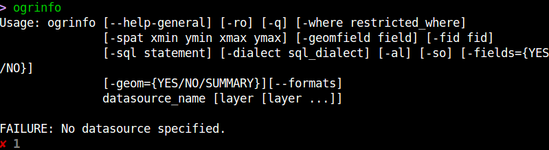
Check point
Exploring Data
Demo Data
Download & unzip
Move data to a "sandbox" directory
Check out the data visually
Use your favorite GIS desktop application to view data
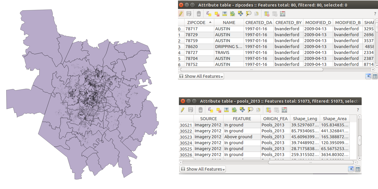
Demo vector data: Austin-area zipcodes & pools
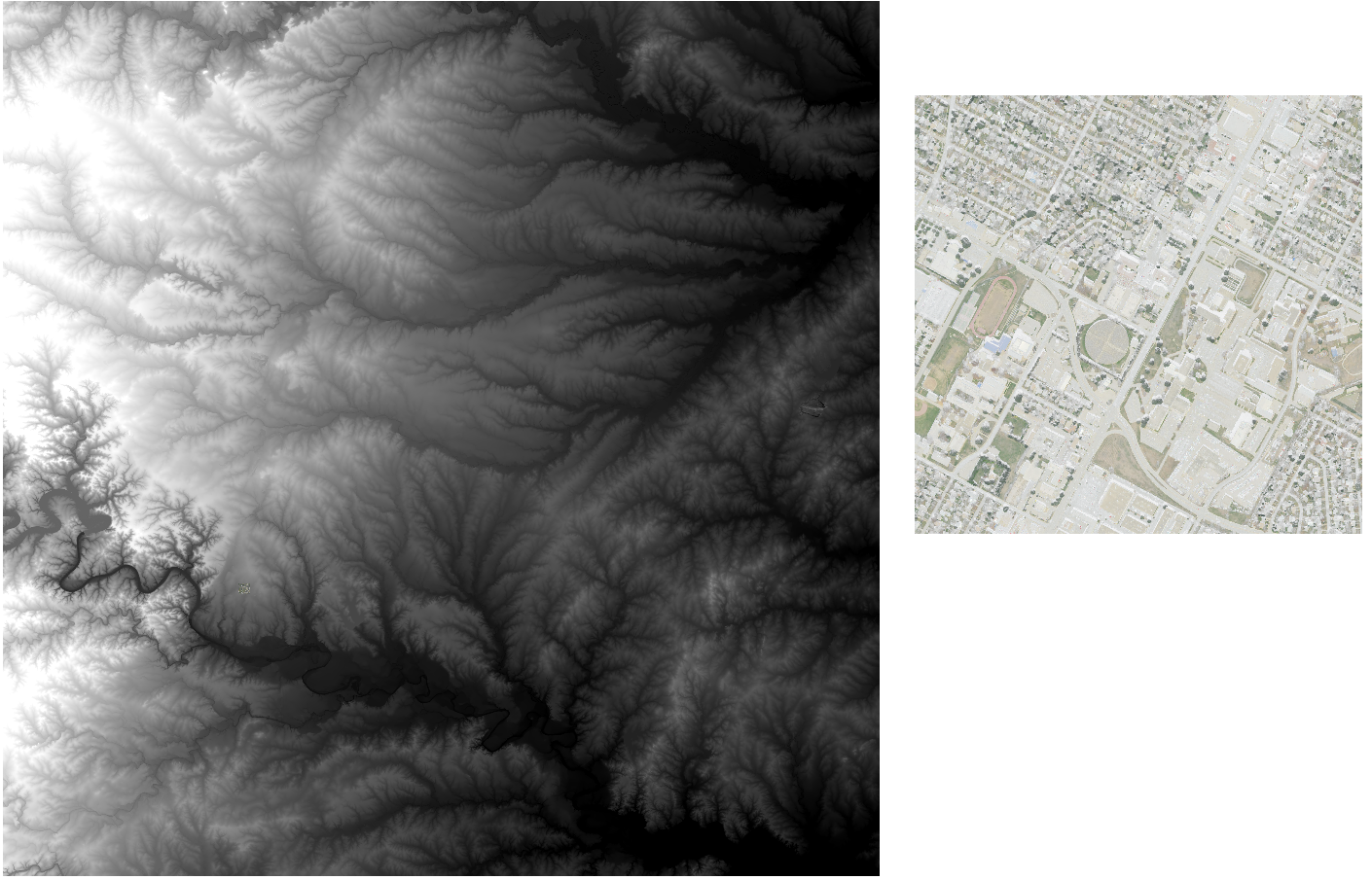
Demo raster data: Austin-area DEM & (clipped) DOQQ
Explore data via the command line
Open your terminal and navigate to your working directory
OGR for vector data
From your working directory, try this:
ogrinfo pools/pools.shp
INFO: Open of `pools/pools.shp'
      using driver `ESRI Shapefile' successful.
1: pools (3D Polygon)
Now try this:
ogrinfo -so zipcodes/zipcodes.shp zipcodes
INFO: Open of `zipcodes/zipcodes.shp'
      using driver `ESRI Shapefile' successful.

Layer name: zipcodes
Geometry: Polygon
Feature Count: 80
Extent: (-98.589809, 29.669673) - (-97.184067, 31.037805)
Layer SRS WKT:
GEOGCS["GCS_WGS_1984",
    DATUM["WGS_1984",
        SPHEROID["WGS_84",6378137,298.257223563]],
    PRIMEM["Greenwich",0],
    UNIT["Degree",0.017453292519943295]]
ZIPCODE: String (12.0)
NAME: String (30.0)
CREATED_DA: Date (10.0)
CREATED_BY: String (50.0)
MODIFIED_D: Date (10.0)
MODIFIED_B: String (50.0)
SHAPE_AREA: Real (19.11)
SHAPE_LEN: Real (19.11)
GDAL for raster data
Try this:
gdalinfo dem10m/dem10m.dem
Driver: USGSDEM/USGS Optional ASCII DEM (and CDED)
Files: dem10m/dem10m.dem
       dem10m/dem10m.dem.aux.xml
Size is 3600, 3600
Coordinate System is:
GEOGCS["NAD83",
    DATUM["North_American_Datum_1983",
        SPHEROID["GRS 1980",6378137,298.257222101,
            AUTHORITY["EPSG","7019"]],
        TOWGS84[0,0,0,0,0,0,0],
        AUTHORITY["EPSG","6269"]],
    PRIMEM["Greenwich",0,
        AUTHORITY["EPSG","8901"]],
    UNIT["degree",0.0174532925199433,
        AUTHORITY["EPSG","9108"]],
    AUTHORITY["EPSG","4269"]]
Origin = (-97.999999407110110,31.000000503864648)
Pixel Size = (0.000277777777778,-0.000277777777778)
Metadata:
  AREA_OR_POINT=Point
Corner Coordinates:
Upper Left  ( -97.9999994,  31.0000005) ( 98d 0' 0.00"W, 31d 0' 0.00"N)
Lower Left  ( -97.9999994,  30.0000005) ( 98d 0' 0.00"W, 30d 0' 0.00"N)
Upper Right ( -96.9999994,  31.0000005) ( 97d 0' 0.00"W, 31d 0' 0.00"N)
Lower Right ( -96.9999994,  30.0000005) ( 97d 0' 0.00"W, 30d 0' 0.00"N)
Center      ( -97.4999994,  30.5000005) ( 97d30' 0.00"W, 30d30' 0.00"N)
Band 1 Block=3600x3600 Type=Float32, ColorInterp=Undefined
  Min=79.900 Max=398.900
  Minimum=79.900, Maximum=398.900, Mean=193.121, StdDev=63.589
  NoData Value=-32767
  Unit Type: m
  Metadata:
    STATISTICS_MAXIMUM=398.89999389648
    STATISTICS_MEAN=193.12105660542
    STATISTICS_MINIMUM=79.900001525879
	STATISTICS_STDDEV=63.588582941289
Converting Data
Exporting original data into new formats
Vector I/O Formats
ogr2ogr --formats
Raster I/O Formats
gdal_translate --formats
shapefile → geojson
let's make a webmap-friendly version
of our zipcodes shapefile:
ogr2ogr -f geojson zipcodes.geojson zipcodes/zipcodes.shp
NOTE: This will generate Warnings - that's ok!
Now try:
ogrinfo zipcodes.geojson
and:
ogrinfo -so zipcodes.geojson OGRGeoJSON
GeoTIFF → georeferenced PNG
gdal_translate -of png doqq.tif converted_doqq.png
Now try:
gdalinfo converted_doqq.png
Reprojecting Data
Side note: EPSG Codes
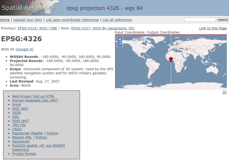 spatialreference.org (great resource!)
Let's make everything WGS84!
ogr2ogr -t_srs EPSG:4326 reprojected_pools.shp
			pools/pools.shp
gdalwarp -t_srs EPSG:4326 doqq.tif reprojected_doqq.tif
Questions so far?
- ogrinfo
- gdalinfo
- ogr2ogr
- gdal_translate
- gdalwarp
Querying Data
Asking questions about your data layers
OGR allows you to use a dialect of SQL ("OGR SQL") to query layers
Q: "How many swimming pools are in Austin?"
ogrinfo pools/pools.shp -sql "SELECT COUNT(*) FROM pools"
INFO: Open of `pools/pools.shp'
      using driver `ESRI Shapefile' successful.

Layer name: pools
Geometry: None
Feature Count: 1
Layer SRS WKT:
(unknown)
COUNT_*: Integer (0.0)
OGRFeature(pools):0
  COUNT_* (Integer) = 51073
A: 51,073
Q: "What is the first pool feature?"
ogrinfo -q pools/pools.shp -sql "SELECT * FROM pools WHERE fid = 1"
Layer name: pools
OGRFeature(pools):1
  POOLS_2013 (Integer) = 2
  CREATED_BY (String) = AeroMetric
  CREATED_DA (Date) = 2013/10/01
  MODIFIED_B (String) = (null)
  MODIFIED_D (Date) = (null)
  SOURCE (String) = LiDAR 2012
  FEATURE (String) = Above ground
  ORIGIN_FEA (String) = Pools_2013
  Shape_Leng (Real) = 44.08991859810
  Shape_Area (Real) = 154.55091064300
  POLYGON ((3164378.2166 9997997.05799999833 0,3164378.178199999034 9997996.324100002646446 0,3164378.063000001013279 9997995.598399996757507 0,3164377.873099997639656 9997994.888400003314018 0,3164377.6096 9997994.202399998903275 0,3164377.275899998844 9997993.547899998724461 0,3164376.875699996948242 9997992.931400001049042 0,3164376.413400001823902 9997992.3605 0,3164375.893700003623962 9997991.840800002217293 0,3164375.322499997913837 9997991.378300003707409 0,3164374.706399999559 9997990.978 0,3164374.0515 9997990.6446999982 0,3164373.365500003099442 9997990.3812 0,3164372.655900001525879 9997990.19089999795 0,3164371.930200003087521 9997990.076099999249 0,3164371.196199998259544 9997990.037399999797 0,3164370.462300002574921 9997990.076099999249 0,3164369.736599996685982 9997990.19089999795 0,3164369.0269 9997990.3812 0,3164368.340599998831749 9997990.644299998879433 0,3164367.686099998652935 9997990.978 0,3164367.0696 9997991.378300003707409 0,3164366.4987 9997991.840800002217293 0,3164365.979000002145767 9997992.360200002789497 0,3164365.516800001263618 9997992.931400001049042 0,3164365.1162 9997993.547499999404 0,3164364.782899998128414 9997994.202399998903275 0,3164364.5194 9997994.888400003314018 0,3164364.329099997878075 9997995.59809999913 0,3164364.214299999177 9997996.324100002646446 0,3164364.175899997353554 9997997.0577 0,3164364.214299999177 9997997.791599996387959 0,3164364.329099997878075 9997998.517300002276897 0,3164364.5194 9997999.227300003170967 0,3164364.782899998128414 9997999.9133 0,3164365.1162 9998000.567900002002716 0,3164365.516500003635883 9998001.184299997985363 0,3164365.979000002145767 9998001.755199998617172 0,3164366.498400002717972 9998002.274899996817112 0,3164367.0696 9998002.737499997019768 0,3164367.686099998652935 9998003.137699998915195 0,3164368.340599998831749 9998003.471100002527237 0,3164369.026600003242493 9998003.734499998390675 0,3164369.736599996685982 9998003.924800001084805 0,3164370.462300002574921 9998004.039599999785 0,3164371.196199998259544 9998004.0784 0,3164371.929799996316433 9998004.039599999785 0,3164372.655900001525879 9998003.924800001084805 0,3164373.365500003099442 9998003.734499998390675 0,3164374.0515 9998003.4714 0,3164374.706399999559 9998003.137699998915195 0,3164375.322499997913837 9998002.737499997019768 0,3164375.893700003623962 9998002.274899996817112 0,3164376.413099996745586 9998001.755500003695488 0,3164376.875699996948242 9998001.184299997985363 0,3164377.275899998844 9998000.567900002002716 0,3164377.6096 9997999.9133 0,3164377.872699998319149 9997999.227300003170967 0,3164378.063000001013279 9997998.517700001597404 0,3164378.178199999034 9997997.791599996387959 0,3164378.2166 9997997.05799999833 0))
Q: "How many above ground pools in Austin?"
ogrinfo -q pools/pools.shp -sql "SELECT COUNT(*) FROM pools WHERE FEATURE = 'Above ground'"
Layer name: pools
OGRFeature(pools):0
  COUNT_* (Integer) = 21550
A: 21,550
Saving query results to a new file
Similar to how you might save a "query view" in other GIS software, you can use OGR to create a new file based on a SQL query
"Create a shapefile containing only the zipcode boundaries in Austin city limits"
ogr2ogr austin_zips.shp zipcodes/zipcodes.shp -sql "SELECT * FROM zipcodes WHERE name = 'Austin'"
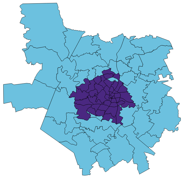 austin_zips.shp (in purple)
"Create a shapefile containing small zipcodes"
ogr2ogr under_10mil.shp zipcodes/zipcodes.shp -sql "SELECT * FROM zipcodes WHERE SHAPE_AREA <10000000"
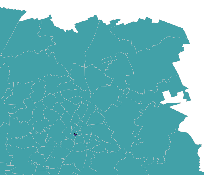
under_10mil.shp (tiny, purple shape)
"Create a geoJSON with only zipcode 78756's boundary"
ogr2ogr -f geojson 78756.geojson zipcodes/zipcodes.shp -sql "SELECT * FROM zipcodes WHERE ZIPCODE = '78756'"
Break
Clipping to create new data
You can clip a target data layer to a given clipping layer to create a new layer
"Create a new layer with only the pools in zipcode 78756"
ogr2ogr -clipsrc 78756.geojson 78756_pools.shp reprojected_pools.shp
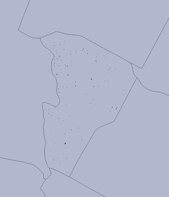
78756_pools.shp (shown over zipcodes)
"Show only the imagery in zipcode 78756"
gdalwarp -cutline 78756.geojson doqq.tif 78756_doqq.tif
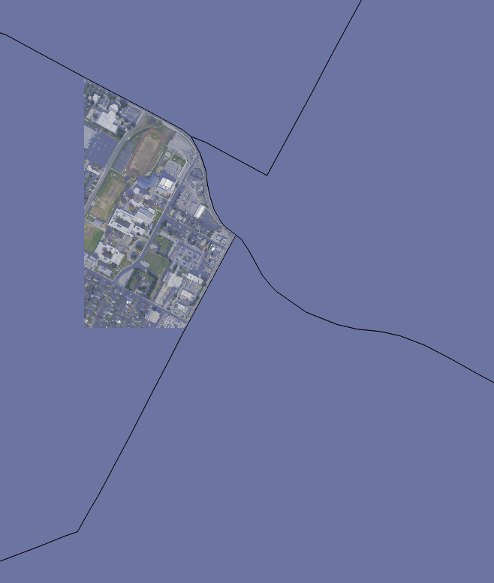
78756_doqq.tif (shown over zipcodes)
"Clip a DEM to a bounding box"
gdal_translate -srcwin 0 0 1000 1000 -of USGSDEM dem10m/dem10m.dem clipped_dem.dem
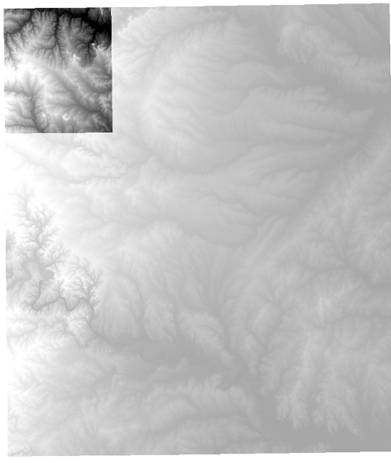
clipped_dem.dem (shown with original DEM)
Fun with DEMs
Now that our DEM is clipped to a more managable size, let's see what it can do
"Generate a hillshade from our DEM"
gdaldem hillshade -of png clipped_dem.dem hillshade.png
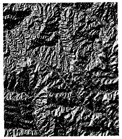
hillshade.png
"Make a hillshade with a different light angle"
gdaldem hillshade -of png -az 135 clipped_dem.dem hillshade135.png
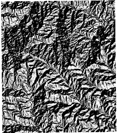
hillshade135.png
"Make a color relief"
gdaldem color-relief clipped_dem.dem colorramp.txt colorrelief.tif
Format of colorramp.txt:
(value) (R) (G) (B)
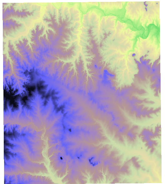
colorrelief.tif
"Create contour lines from a DEM"
gdal_contour -a elev -i 20 clipped_dem.dem contours.shp
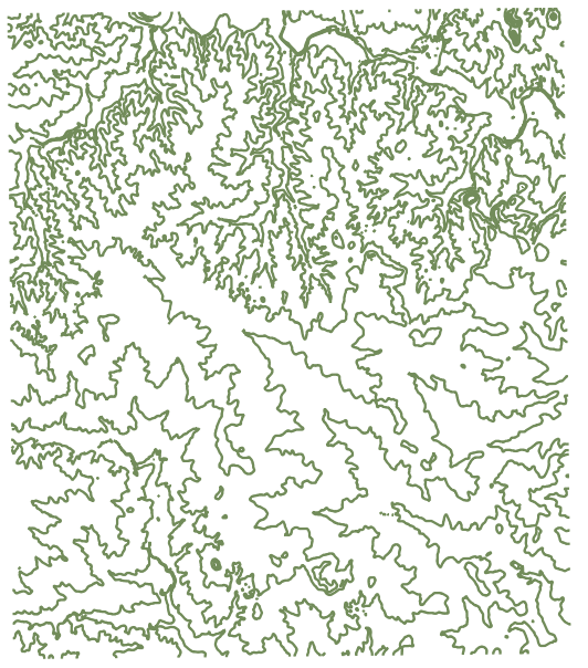
contours.shp
Questions?
Thank you!!!
saras.link/gdal_slides
sara@hartsafavi.com | sasha@hartsafavi.com
Things to Try on Your Own
Googling is good! Or check the useful links on next slide.
- Reproject a dataset using a PROJ4 string or a .prj file
- Create an index on the zipcodes shapefile
- Merge two datasets together
- Resize a raster
Useful Links
https://github.com/dwtkns/gdal-cheat-sheet
http://www.gdal.org/ogr_sql.html
http://www.gdal.org/gdal_utilities.html